Statistical Learning
A Review on Computer Vision Fundamentals
Introduction
You have probably seen this thing floating around in several machine learning courses: \(P(y|x,\theta)\), \(P(\theta|x,y)\), or even the term MAP and MLE. If you haven’t yet, you will probably start seeing them after. These concepts comes from statistics where they’re called statistical learning, parameter estimation, probabilistic inference, or one of their many synonyms. But what are they? How do they relate to vision? And why is it useful to think about them?
Let us start with a toy example. We want to design an autonomous system to tell when the car should go or stop, depending on the traffic light. Our dataset are pictures of traffic lights and we want our model \(M(\theta)\) to classify whether an image is \(\text{GO}\) or \(\text{STOP}\) parameterized by \(\theta\). Using one-hot encoding, we let \(\mathbf{y}_i:=\begin{bmatrix} 1 & 0 \end{bmatrix}^\top\) for \(\text{GO}\) and \(\mathbf{y}_i:=\begin{bmatrix} 0 & 1 \end{bmatrix}^\top\) for \(\text{STOP}\). Let red and yellow light be \(\text{STOP}\) and green light be \(\text{GO}\) for our intents and purposes.
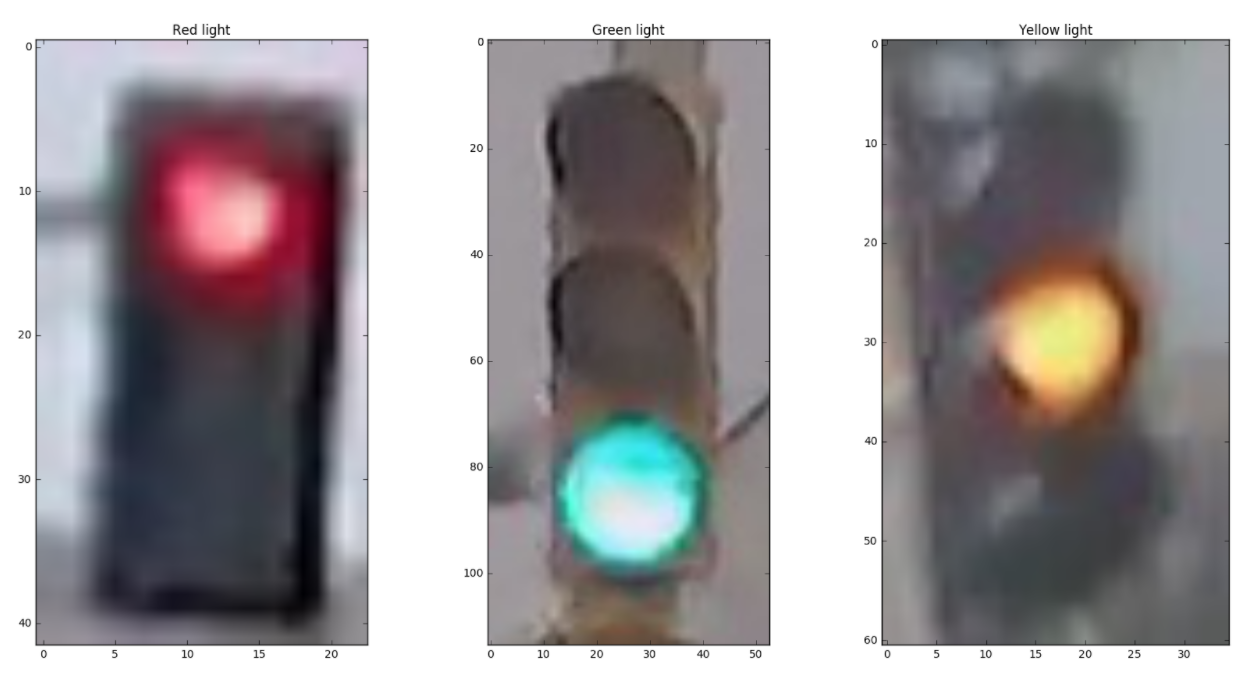
To simplify our case even more, let us abstract away the high-dimensional input of an image and let \(\mathbf{x}_i:=\begin{bmatrix} x_r & x_y & x_g \end{bmatrix}^\top\), where each component \(\in[0,1]\) corresponds to a snapshot of the illumination intensity of red \(x_r\), yellow \(x_y\), and the green \(x_g\) bulb of a traffic light. So, we can visualize our data as…
Now that we have introduced our scenario, let us get into the main idea of this blog.
Learners
For any ML-based vision models (really any vision models you come across now,) we have a learner and a model, as explained in Torralba, Isola, and Freeman (2024, chap. 9). A model can be neural networks, transformers, etc… but we will do something simpler. But first, what kind of learner are we trying to model here? Is it supervised, self-supervised, unsupervised, or reinforcement learning? Is it a generative or discriminative learning? 2
2 After the generative model boom, this distinction has become more important. Generative model has long existed in statistics, and has only been recently (within 5 years) exposed to the vision community at a scale.
3 Since there are only two categories, we can simplify it to a binary classification; however, multi-class classification generalizes to any \(K\) categories, it will be more easier to visualize how it works. Single-label just means the categories are mutually exclusive, and the model should expect to output a single category per input sample (i.e., image).
Since we already have a pretty clear \(\mathbf{x}\) and \(\mathbf{y}\), it probably means we are working under a supervised learning regime. We want our model to predict \(\mathbf{y}\), so it would also be under supervised discriminative learning regime. Since our labels for \(\mathbf{y}\) are categorical, we will specifically be working with multi-class (single-label) classifiers 3.
Before continuiting, please refer to Murphy (2012, chap. 3.2) to know more about Bayes’ theorem and how likelihoods, posteriors, priors, and evidence all have special meaning and nuances despite them denoted as \(p\) for probabilities.
4 If you known gradient descent and the notion of “loss” in ML/vision, the following three approaches are a generalization to them. These general form allows us to see learning at a bigger picture, though we won’t be discussing this here.
According to S. J. D. Prince (2012, chap. 4), there are three classical approaches for supervised discriminative learning4:
Maximum Likeilhood Estimation (MLE)
\(\hat{\theta}=\arg\max_{\theta}p(\mathbf{y}|\mathbf{x},\theta)\)
Remember, \(\mathbf{y}\) and \(\mathbf{x}\) are our training data and cannot be changed. The only thing we can (and should) change is the model parameter \(\theta\). So, this is basically saying what value of \(\theta\) can maximize the probability of the correct label \(\mathbf{y}\) from its corresponding input \(\mathbf{x}\) for all samples (i.e., data points). The \(p(\mathbf{y}|\mathbf{x},\theta)\) is known as the likelihood of \(\theta\). We will define what \(\theta\) is later, but basically it is an abstract representation of model’s parameter, representing choices of hypothesis that best explains data relationship.
Maximum a Posteriori (MAP) Estimation
\(\hat{\theta}=\arg\max_{\theta}p(\theta|\mathbf{x},\mathbf{y})=\arg\max_{\theta}\frac{p(\mathbf{y}|\mathbf{x},\theta)p(\theta)}{p(\mathbf{x},\mathbf{y})}\propto \arg\max_{\theta}p(\mathbf{y}|\mathbf{x},\theta)p(\theta)\)
This is saying which parameter \(\theta\) for our model (i.e., weights) has the highest probability that explains the data relationship between \(\mathbf{x}\) and \(\mathbf{y}\). In other words, this maximizes the posterior distribution \(P(\theta|\mathbf{x},\mathbf{y})\) (i.e., the posterior of \(\theta\)). We then use the Bayes’ theorem 5 to get back our likelihood again with an additional prior \(p(\theta)\) 6 with a constant factor \(\frac{1}{p(\mathbf{x},\mathbf{y})}\) which can be ignored 7.
5 A commonly used special operation in statistics/probabilities. Check here
6 There’s many ways to think about prior \(p(\theta)\). You think of it as a weighting factor of the likelihood that says how likely that likelihood is given the selected \(\theta\). Or, as a balance between data-driven likelihood and previously known (i.e., “prior”) knowledge on how \(\theta\) should behave (e.g., \(\theta\) is likely to be 67 for some reason). Or, as a regularizer where we follow Occam’s razor that the weights should be simple.
7 This is a probability over the training data \(\mathbf{y}\) and \(\mathbf{x}\). It’s not going to change throughout the maximization process of \(\theta\).
Bayesian Inference
\(p(y^*|x^*,\mathbf{x},\mathbf{y})=\int p(y^*|x^*,\theta)p(\theta|\mathbf{x},\mathbf{y})d\theta\)
Instead of estimating a specific parameter \(\theta\) (i.e., point estimate), we interpret the model’s parameters \(\theta\) as probabilistic 8. Notice we are not maximizing anything or even calculating \(\theta\) itself, but directly predicting our unseen data point \(y^*\) given \(x^*\). In fact, this is a summation of each prediction \(p(y^*|x^*,\theta)\) from all possible parameter \(\theta\) weighted by the posterior for each \(\theta\). The integral can sometimes be computed analytically given a good conjugate prior 9, but most of the time, it is approximated by sampling (i.e., Monte-Carlo).
8 In statistics, there are two interpretations: frequentist (there’s a single true value and the randomness is strictly from sampling error like MLE/MAP) and Bayesian (there are no true value and the probability is intrinsic).
9 A special prior when combined with its corresponding likelihood produces a nice-to-work-with analytical posterior (remember, we are integrating the posterior, which is nasty most of the time). For example, the Gaussian distribution \(\mathcal{N}(\mu,\sigma^2)\)’s conjugate prior is Normal-inverse gamma. Check here.
Others
For generative or unsupervised models, we don’t necessarily have a label \(\mathbf{y}\). What we do instead is have the model learn the data distribution of the input \(\mathbf{x}\) itself, resulting in posteriors with \(p(\theta|\mathbf{x})\) instead of \(p(\theta|\mathbf{x},\mathbf{y})\), or likelihood of \(p(\mathbf{x}|\theta)\) instead of \(p(\mathbf{y}|\mathbf{x},\theta)\). Sometimes, they also have the latent distribution \(\mathbf{z}\) as a more efficient, intermediate way to have the model learn the distribution. For example, VAEs Simon J. D. Prince (2023, chap. 17.3) and diffusions Simon J. D. Prince (2023, chap. 18.4) are learned via MLE with \(p(\mathbf{x}|\theta)\) as the likelihood. In some cases, we do a maximization and a minimization of two different sets of parameters \(\theta\) and \(\phi\) like in GANs Simon J. D. Prince (2023, chap. 15.1.1). Or, in Deep RL, we maximize the policy Simon J. D. Prince (2023, chap. 19.3).
For the purpose of learning (i.e., you learning this), we will stick with much more simpler MLE under supervised discriminative learning. Now enough with the theory and see some visuals from our example scenario.
Example: MLE for multi-label classification
Let us first visualize our data.
Our likelihood \(p(\mathbf{y}|\mathbf{x},\theta)\) will follow a categorical distribution where \(p(\mathbf{y}_i=\mathbf{k}|\mathbf{x}_i,\theta)\) denotes the likelihood for each data sample \(i\) and \(\mathbf{k}\in K=\{\text{STOP},\text{GO}\}\), where \(K\) can be thought of as a set of all one-hot-encoded categories. 10
10 Think of it like a vector-valued likelihood where \(p(\mathbf{y}_i|\mathbf{x}_i,\theta)=\begin{bmatrix} p(\mathbf{y}_i= & \text{GO} & |\mathbf{x}_i,\theta) \\ p(\mathbf{y}_i= & \text{STOP} & |\mathbf{x}_i,\theta) \end{bmatrix}\)
Now, to choose a model, we will use multivariate Gaussian distribution to represent each categories. Remember, the model we choose are arbitrary and mostly follows what we think is the best for the given situation. We might choose logistic regression for a binary classification (which is still slightly different from two-label classification) to decide whether an image of a light is \(\text{GO}\) or \(\text{STOP}\). Or, we can follow one of the more later trends and use neural networks on everything. But overall, it doesn’t change the overall theory of learning and the underlying optimization and criterion/loss, so we pick the simpler option: multivariate Gaussian distribution.
Recall, a univariate Gaussian \(\mathcal{N}(x|\mu, \sigma^2)=\frac{1}{\sqrt{2\pi\sigma^2}}e^{-\frac{(x-\mu)^2}{2\sigma^2}}=\frac{1}{\sqrt{(2\pi)^1\sigma^2}}e^{-\frac{1}{2}(x-\mu)(\sigma^2)^{-1}(x-\mu)}\). However, our input is 3D, so we have to use 3D multivariate Gaussian \(\mathcal{N}_3(\mathbf{x}|\mathbf{\mu}, \Sigma)=\frac{1}{\sqrt{(2\pi)^3|\Sigma|}}e^{-\frac{1}{2}(\mathbf{x}-\mathbf{\mu})^\top\Sigma^{-1}(\mathbf{x}-\mathbf{\mu})}\)11. In other words, we let \(p(\mathbf{x}_i|\mathbf{y}_i=\mathbf{k},\theta):=\mathcal{N}_3(\mathbf{x}_i|\mathbf{\mu}_\mathbf{k}, \Sigma_\mathbf{k})\).
11 For more info on multivariate Gaussian and the covariance matrix \(\Sigma\), check Simon J. D. Prince (2023, Appendix C.3.2)
Now let’s go check what’s the initial default distribution the model has started with.
Basically, we want these distributions to match (so the model is able to classify correctly), which currently it is not.
Given \(\theta=\{\mu_\text{GO}, \Sigma_\text{GO}, \phi_\text{GO}, \mu_\text{STOP}, \Sigma_\text{STOP}, \phi_\text{STOP}\}\)12, we can finally define our MLE exactly as \[ \begin{align} \arg\max_\theta \frac{1}{n}\sum^n_{i=1} p(\mathbf{y}_i=\mathbf{k}|\mathbf{x}_i,\theta) &= \arg\max_\theta \frac{1}{n}\sum^n_{i=1} \frac{p(\mathbf{y}_i=\mathbf{k},\mathbf{x}_i|\theta)}{p(\mathbf{x}_i|\theta)} \\ &= \arg\max_\theta \frac{1}{n}\sum^n_{i=1} \frac{p(\mathbf{x}_i|\mathbf{y}_i=\mathbf{k},\theta)p(\mathbf{y}_i=\mathbf{k}|\theta)}{\sum_{\mathbf{j}\in K} p(\mathbf{x}_i|\mathbf{y}_i=\mathbf{j},\theta)p(\mathbf{y}_i=\mathbf{j}|\theta)} \\ &= \arg\max_\theta \frac{1}{n}\sum^n_{i=1} \frac{\mathcal{N}_3(\mathbf{x}_i|\mathbf{\mu}_\mathbf{k}, \Sigma_\mathbf{k}) p(\mathbf{y}_i=\mathbf{k}|\theta)}{\sum_{\mathbf{j}\in K} \mathcal{N}_3(\mathbf{x}_i|\mathbf{\mu}_\mathbf{j}, \Sigma_\mathbf{j})p(\mathbf{y}_i=\mathbf{j}|\theta)} \end{align} \] 13
12 For each one-hot-encoded category \(\mathbf{k}\in K\), \(\mu_\mathbf{k}\) and \(\Sigma_\mathbf{k}\) represents the model’s parameter for each of the categories’ Normal distribution (mean and variance, respectively). \(\phi_\mathbf{k}\) represents the ratio/weighting of each category \(\mathbf{k}\). So, \(p(\mathbf{y}_i=\mathbf{k}|\theta)=\phi_\mathbf{k}\)
13 \[ \begin{align} p(a,b|c) &= \frac{p(a,b,c)}{p(c)} \\ &= \frac{p(a,b,c)p(b,c)}{p(c)p(b,c)} = \frac{p(a,b,c)}{p(b,c)}\frac{p(b,c)}{p(c)} \\ &= p(a|b,c)p(b|c) \end{align}\]
14 The GDA/QDA, despite its name, actually has to go through a generative hoop for the derivation, since we are actually modelling our input \(\mathbf{x}_i\) as some distribution which we can technically re-sample from again to generate a new sample of the similiar distribution to \(\mathbf{x}_i\).
In fact, learning a model where we assume the \(\mathbf{x}\)’s in each category of the categorical distribution \(\mathbf{y}\) as a Gaussian is known as Gaussian Discriminative Analysis (GDA) or Quadratic Discriminative Analysis (QDA) which can you read more here. Additionally, this is very close to the most well-known model/learner out there: Naïve Bayes. Naïve Bayes assumes each input data point \(\mathbf{x}_i\) are independent of each other, but GDA/QDA assumes each input data point \(\mathbf{x}_i\) follow a Gaussian distribution as mentioned before. 14
Analytical Estimation of \(\theta\)
Since GDA/QDA are clean to work with, they have an analytical method to compute the optimal parameter \(\theta\) given the data \(\mathbf{x}\) and \(\mathbf{y}\). We basically compute the derivative of the log-likelihood with respect to each parameters to obtain the following 15.
15 Check the derivations here
We find that \(\phi_k=\frac{n_\mathbf{k}}{n}\) where \(n\) is the total number of samples/data while \(n_\mathbf{k}\) is the number of samples with \(\mathbf{y}_i=\mathbf{k}\).
\[ \begin{align} \mathbf{\mu}_\mathbf{k} &= \frac{\sum_{i \text{ s.t. } \mathbf{y}_i=\mathbf{k}} \mathbf{x}_i}{n_\mathbf{k}} \\ \Sigma_\mathbf{k} &= \frac{\sum_{i \text{ s.t. } \mathbf{y}_i=\mathbf{k}} (\mathbf{x}_i-\mathbf{\mu}_\mathbf{k})(\mathbf{x}_i-\mathbf{\mu}_\mathbf{k})^\top}{n_\mathbf{k}} \\ \end{align} \]
Gradient Descent Estimation of \(\theta\)
Since we are using QDAs/GDAs, we have analytical solution available us (and we should use it in practice if QDAs/GDAs is what we really want). But most ML models, especially in vision, uses more complicated formulations like neural networks, we have to resort using numerical optimizations like gradient descent (GD), stochastic gradient descent, and Adam. So let us see how we optimize model in the majority of the cases via GD over the negative log-likelihood (NLL), which is just the negation of the log of the likelihood \(\frac{1}{n}\sum^n_{i=1} p(\mathbf{y}_i=\mathbf{k}|\mathbf{x}_i,\theta)\), including the NLL of the Gaussian in def neg_log_likelihood_gaussian. Note, we omit \(\log\phi_\mathbf{k}\) since we are not optimizing that.
This will take about a few minutes. Make sure you run the previous cell.
You can see how the model distribution gets closer to the true data distribution for each gradient step. Remember, each point is a data point representing the 3-pixel image of a traffic light. Theoretically speaking, if there exists an analytical solution of a quadratic expression (single minimum), gradient descent should effectively reach to the same optimal point. However, the reason it’s not is likely because we’re missing the class prior \(\phi_\mathbf{k}\) or the variance (i.e., the spread) is different between the two categories (needing two different learning rate?) Regardless, it still mostly converges.
Summary
Overall, you saw a simple GDA model to classify a 3-pixel image input of a traffic light as either \(\text{GO}\) or \(\text{STOP}\), which would be used to tell the car to move or not. But if you recall, this is a simple abstraction. In a more realistic setting, we would have our models read from real images (i.e., an actual image of a traffic light), so you can expect the distribution would not just be over 3D (i.e., the three pixels), but one million dimensions! We also get to see how the model themselves is actually just a small part of the greater learning system. Instead of a normal distribution \(\mathcal{N}\), we can replace it with a multi-layered neural networks, or even augment it with convolutional layers, and the main idea still doesn’t change.
So, going back to the original three questions:
- What are they?
MAPs and MLEs are particular learning schemes we can use on our models to estimate an optimal \(\theta\) given \(\mathbf{x}\) and \(\mathbf{y}\). It also has a more general version where \(\theta\) is modelled in a Bayesian/probabilistic way (i.e., Bayesian prediction).
- How do they relate to vision?
Because probabilistic learners are not just restricted to tabular data, allowing other forms of data to train on the model (i.e., images). From a classical vision standpoint, assuming the model and the learning process as probabilistic allows the use of various powerful, abstract tools from statistics to model arbitrary distributions of visual data (i.e., quadratic discriminative analysis), whereas one needs to design different models for different domains. Refer Sutton (2019).
- Why are they useful to think about them?
Nature is too complicated. Probability is likely the best way to effectively model complex processes into something simpler to work with, allowing effective training of the model for seemingly intelligent prediction. Refer Sutton (2019).
More practically, all deep learning-based vision models employs these statistical tools, and even moreso on modern generative models. So, to learn and apply these latest models, one likely needs to have strong foundation in these aspects.