Foggy Cornell Box
Micro Blog: Volumetric Path Tracer
An attempt at creating the most basic volumetric path tracer: Cornell box in foggy atmosphere that is uniformly diffused within the air. Overall concepts will be based on Pharr, Jakob, and Humphreys (2023, chap. 11) and Pharr, Jakob, and Humphreys (2023, chap. 14).
Volumetric Scattering Model
In basic volumetric rendering, there are four more assumptions (on top of surface scattering) based on the underlying physical processes of these three main 1 types of light interaction with participating media 2: absorption, emission, and scattering.
1 Chandrasekhar (2013, chap. 1) nicely put it as “we shall not aim at the maximum generality possible but limit ourselves, rather, by the situations which the problem considered in this book actually required.” So in terms of the theory behind the volumetric light transport in participating media itself, it really is just these four main types of interaction to consider. Anything else is likely unnecessarily complicated.
2 Volumetric rendering is not necessarily associated with participating media. You can do volumetric rendering on surface-only scenes, but that would unnecessarily complicate and slow-down the rendering.
1st assumption: Absorption. \(dL_o(\mathbf{x},\omega)=-\sigma_a(\mathbf{x},\omega)L_i(\mathbf{x},-\omega) dt\)
2nd assumption: Emission3. \(dL_o(\mathbf{x},\omega)=\sigma_a(\mathbf{x},\omega)L_i(\mathbf{x},-\omega) dt\)
3 According to Chandrasekhar (2013, chap. 4), the emission of the participating media uses the same absorption coefficient, except negated, since Kirchhoff’s law states the absorbing media must be at thermal equilibrium, which means it also needs to emit at the same rate to ensure the media does not keep gaining energy, unless externally sourced (which we assume not for now).
4 One might ask if in-scattering has a phase function, why does out-scattering not have a phase function? Chandrasekhar (2013, chap. 3) actually shows out-scattering does, but it does not depend on the variation of radiance (i.e., intensity and color), since there’s only one kind of intensity and color, it merely reduced down to the coefficient \(\sigma_s\).
3rd assumption: Out-scattering4. \(dL_o(\mathbf{x},\omega)=-\sigma_s(\mathbf{x},\omega)L_i(\mathbf{x},-\omega) dt\)
This is one of two types of scattering that models the reduction of radiance along a ray when it scatters away from the direction of the ray.
4th assumption: In-scattering. \(\displaystyle dL_o(\mathbf{x},\omega)=\sigma_s(\mathbf{x},\omega)\int_{S^2}p(\mathbf{x},\omega_i,\omega)L_i(\mathbf{x},\omega_i)d\omega_i\)
This is the other type of scattering that models the increase of radiance along a ray when it scatters into the direction of the ray.
Notice that absorption and out-scattering removes radiance while emission and in-scattering adds radiance. We group absorption and out-scattering together into attenuation/extinction coefficient \(\sigma_\text{t}=\sigma_a+\sigma_s\) that describes the overall reduction of the radiance along the ray (i.e., \(dL_o(\mathbf{x},\omega)=-\sigma_\text{t}(\mathbf{x},\omega)L_i(\mathbf{x},-\omega) dt\)). Additionally, we also have a single-scattering albedo, \(\rho(\mathbf{x},\omega)=\frac{\sigma_s(\mathbf{x},\omega)}{\sigma_\text{t}(\mathbf{x},\omega)}\), which describes the ratio on how much it scatters rather than absorbed. As for the other two, we merge both in-scattering and emission into \(dL_o(\mathbf{x},\omega)=\sigma_\text{t}(\mathbf{x},\omega)L_s(\mathbf{x},\omega)dt\) where the source function \(L_s\) is \(\displaystyle L_s(\mathbf{x},\omega):=\frac{\sigma_a(\mathbf{x},\omega)}{\sigma_\text{t}(\mathbf{x},\omega)}L_e(\mathbf{x},\omega)+\rho(\mathbf{x},\omega)\int_{S^2}p(\mathbf{x},\omega_i,\omega)L_i(\mathbf{x},\omega_i)d\omega_i\).
We will first assume the fog is a perfect scattering of a participating media with isotropic scattering5 (i.e., no absorption; no emission; constant phase function) So how does one even render it?
5 Isotropic media is not the same as isotropic phase function, where the former refers particles with uniform arrangements or having a very round shape while the latter refers to whether the full-spherical scattering is uniform.
Now, before we get to that, there’s more intermediate structure we have to build. Currently, these fundamental assumption of volumetric physical processes are defined via differential equations, since these processes constantly involves with the spatial medium that permeates the “air” as it traverses through it. This makes diff. eqs. a natural description of how a ray incrementally change in radiance as it incrementally traverse the media. Modelling surface-only effects (e.g., traditional BSDF) only cares about physical processes at discrete amount of bounces on each surfaces; hence, diff. eqs. is unnecessary. However, most renderer is based on integral formulations since we mostly care about the overall radiance produced before the sensor instead of the local effects of volumetric or surface scattering (in the grand scheme of things). So, we need to somehow convert these diff. eqs. to integrals first in order to apply common rendering algorithms on these new volumetric assumptions.
Transmittance
First, let us look into the extinction portion of the volumetric effects: \(dL_o(\mathbf{x}, \omega) = -\sigma_\text{t}(\mathbf{x}, \omega) L_i(\mathbf{x}, -\omega)dt\), which is more explicitly written as \(dL_o(\mathbf{x}+t\omega, \omega) = -\sigma_\text{t}(\mathbf{x}+t\omega, \omega) L_i(\mathbf{x}+t\omega, -\omega)dt\). When \(t=0\), we are at \(\mathbf{x}\). whereas we denote the location of \(\mathbf{x}'\) along the direction \(\omega\) when the ray has traversed to time \(t\).
\[\begin{align} dL_o(\mathbf{x}+t\omega, \omega) &= -\sigma_\text{t}(\mathbf{x}+t\omega, \omega) L_i(\mathbf{x}+t\omega, -\omega)dt \\ dL_o(\mathbf{x}+t\omega, \omega) &= -\sigma_\text{t}(\mathbf{x}+t\omega, \omega) L_o(\mathbf{x}+t\omega, \omega)dt \end{align}\]
For the sake of brevity, we will abbreviate the notation and re-introduce them later. Pro tip: always use definite integral; indefinite integral causes a lot of confusion in these complicated settings, especially with nested variables like here.
\[\begin{align} dL_o &= -\sigma_\text{t} L_o dt \\ \frac{1}{L_o} \frac{dL_o}{dt} &= -\sigma_\text{t} \\ \int^{t=d}_{t=0} \frac{1}{L_o} \frac{dL_o}{dt} dt &= \int^{t=d}_{t=0} -\sigma_\text{t} dt \\ \int^{L_o(t=d)}_{L_o(t=0)} \frac{dL_o}{L_o} &= \int^{t=d}_{t=0} -\sigma_\text{t} dt \\ \ln{|L_o(t=d)|}-\ln{|L_o(t=0)|} &= \int^{t=d}_{t=0} -\sigma_\text{t} dt \\ \frac{L_o(t=d)}{L_o(t=0)} &= e^{\int^{t=d}_{t=0} -\sigma_\text{t} dt} \\ \frac{L_o(\mathbf{x}+d\omega, \omega)}{L_o(\mathbf{x}, \omega)} &= e^{-\int^{t=d}_{t=0} \sigma_\text{t} dt} \\ \frac{L_o(\mathbf{x}', \omega)}{L_o(\mathbf{x}, \omega)} &= e^{-\int^{t=d}_{t=0} \sigma_\text{t} dt} \\ \end{align}\]
This perfectly matches the book’s definition of transmittance \(T_r(\mathbf{x}\to\mathbf{x}'):=\frac{L_o(\mathbf{x}', \omega)}{L_o(\mathbf{x}, \omega)}\) where it is always between \(0\) and \(1\)6, which will be important for our rendering algorithm as a nice way to encapsulate the idea of absorption and out-scattering as an accumulated transmittance on a point along a ray. This is better related to an idea known as attenuation. Additionally, the exponent in the transmittance, \(-\int^{t=d}_{t=0} \sigma_\text{t} dt\), refers to optical thickness/depth, which just tells us how much the light is scattered or absorbed in total (linearly) different from the exponentiated version that tells us what the actual final radiance produced.
6 Since \(\mathbf{x}'\) represents a point later, or further away, from the light source then \(\mathbf{x}\), its outgoing radiance must at most be the same or reduced, but not negative. Hence, \(T_r\in [0,1]\). Can also be thought of as the fraction between the radiance of the earlier \(\mathbf{x}\) and the later \(\mathbf{x}'\).
The Equation of Transfer
Transmittance only talks about all the processes that involves reducing the radiance, which is only a part of it. What about the rest? One neat thing about all the assumed equations… they all modify/change the same underlying \(L_o\)! So, we can aggregate each of these individual processes into one diff. eq.: \(dL_o(\mathbf{x}+t\omega, \omega) = -\sigma_\text{t}(\mathbf{x}+t\omega, \omega) L_i(\mathbf{x}+t\omega, -\omega)dt + \sigma_\text{t}(\mathbf{x}+t\omega, \omega) L_s(\mathbf{x}+t\omega, \omega)dt\) to be integrated. As usual, we will abbreviate the notation for brevity. When the ray \((\mathbf{x},\omega)\) intersects a surface, we will denote the location of intersection as \(\mathbf{x}_s\) in which the ray has traveled \(t=d\).
\[\begin{align} dL_o &= -\sigma_\text{t} L_idt + \sigma_\text{t} L_sdt \\ dL_o &= -\sigma_\text{t} L_odt + \sigma_\text{t} L_sdt \\ \frac{dL_o}{dt} + \sigma_\text{t} L_o &= \sigma_\text{t} L_s \\ (e^{\int^{s=t}_{s=0} \sigma_\text{t} ds}) \frac{dL_o}{dt} + (e^{\int^{s=t}_{s=0} \sigma_\text{t} ds}) \sigma_\text{t} L_o &= (e^{\int^{s=t}_{s=0} \sigma_\text{t} ds}) \sigma_\text{t} L_s \\ (e^{\int^{s=t}_{s=0} \sigma_\text{t} ds}) \frac{dL_o}{dt} + (e^{\int^{s=t}_{s=0} \sigma_\text{t} ds}) (\frac{d}{dt} \int^{s=t}_{s=0}\sigma_\text{t} ds) L_o &= (e^{\int^{s=t}_{s=0} \sigma_\text{t} ds}) \sigma_\text{t} L_s \\ \int^{t=d}_{t=0} \frac{d}{dt} (e^{\int^{s=t}_{s=0} \sigma_\text{t} ds} L_o) dt &= \int^{t=d}_{t=0} (e^{\int^{s=t}_{s=0} \sigma_\text{t} ds}) \sigma_\text{t} L_s dt \\ e^{\int^{s=d}_{s=0} \sigma_\text{t} ds} L_o(t=d) - e^{\int^{s=0}_{s=0} \sigma_\text{t} ds} L_o(t=0) &= \int^{t=d}_{t=0} (e^{\int^{s=t}_{s=0} \sigma_\text{t} ds}) \sigma_\text{t} L_s dt \\ L_o(t=d) &= e^{-\int^{s=d}_{s=0} \sigma_\text{t} ds} L_o(t=0) + e^{-\int^{s=d}_{s=0} \sigma_\text{t} ds} \int^{t=d}_{t=0} (e^{\int^{s=t}_{s=0} \sigma_\text{t} ds}) \sigma_\text{t} L_s dt \\ L_o(t=d) &= e^{-\int^{s=d}_{s=0} \sigma_\text{t} ds} L_o(t=0) + \int^{t=d}_{t=0} (e^{-\int^{s=d}_{s=t} \sigma_\text{t} ds}) \sigma_\text{t} L_s dt \\ L_o(t=d) &= T_r(\mathbf{x}\to\mathbf{x}_s) L_o(t=0) + \int^{t=d}_{t=0} T_r(\mathbf{x}'\to\mathbf{x}_s) \sigma_\text{t} L_s dt \end{align}\]
However, this is calculated in the direction towards the point of intersection starting from \(\mathbf{x}\). For the sake of convention, we will reformulate this as a ray marching towards the surface intersection but pointing back to \(\mathbf{x}\) by negating the direction \(\omega\) as a way to compute the incoming radiance \(L_i\) at \(\mathbf{x}\) from the surface intersection (and all the volumetric effects that occurs in-between). The equation can be intuitively understood as summing the incremental volumetric effects from the attenuated incoming radiance along the ray (i.e., line integral) and the additional effects from the surface scattering attenuated at the entire length. 7
7 Note, the book uses \(\sigma_\text{t}(\mathbf{x}',\omega)\) with the un-negated direction \(\omega\) likely from different parameterization. However, as long as the attenuation coefficient is directionally symmetric, \(\sigma_\text{t}(\mathbf{x}',\omega)=\sigma_\text{t}(\mathbf{x}',-\omega)\), which occurs in most basic volumetric media, then this discrepancy can be ignored with discretion.
The Equation of Transfer (Integral Form):
\[ L_i(\mathbf{x},\omega) = T_r(\mathbf{x}_s\to\mathbf{x}) L_o(\mathbf{x}_s,-\omega) + \int^{t=d}_{t=0} T_r(\mathbf{x}'\to\mathbf{x}) \sigma_\text{t}(\mathbf{x}',-\omega) L_s(\mathbf{x}',-\omega) dt \]
Another important idea is when there are no surface scattering along the path the ray travels. Then, \(d\to\infty\), \(\mathbf{x}_s\) is undefined, and no surface scattering at \(d\) to emit the first term of The Equation of Transfer.
Volumetric Light Transport
Now, we have all the necessary diff. eqs. converted into integral form, we can try incorporating volumetric effects into our core rendering algorithm. But before we do that (I know), our current formulation only supports local light transport since it only specifies for a single ray (i.e., no bounce). Now, we have to extend them into the path-space integral formulation for supporting global light transport (i.e., multi-bounce).
While the book provides the full theoretical generalization of volumetric path integral, it doesn’t tell us how we should implement our own renderer in a clear way. We will re-devise our own formulation that closely resembles the rendering algorithm itself with next-event estimation (NEE). 8 To simplify the formulation, we will apply our own assumption of the sampling process to simplify the math & the algorithm while keeping the accuracy of our rendering.
8 It is important to get a good looking rendering that is simple, fast, and unbiased. NEE should do the job in the volumetric case.
Recall our equation of transfer and the source function \(L_s\):
\[ L_i(\mathbf{x},\omega) = T_r(\mathbf{x}_s\to\mathbf{x}) L_o(\mathbf{x}_s,-\omega) + \int^{t=d}_{t=0} T_r(\mathbf{x}'\to\mathbf{x}) \sigma_\text{t}(\mathbf{x}',-\omega) L_s(\mathbf{x}',-\omega) dt \] \[ L_s(\mathbf{x},\omega):=\frac{\sigma_a(\mathbf{x},\omega)}{\sigma_\text{t}(\mathbf{x},\omega)}L_e(\mathbf{x},\omega)+\rho(\mathbf{x},\omega)\int_{S^2}p(\mathbf{x},\omega_i,\omega)L_i(\mathbf{x},\omega_i)d\omega_i \]
Simplifying results until we get a recursive form in \(L_i\) (which depends on \(\omega_i\)) 9:
9 We assume BRDF (no BTDF) for our BSDF.
\[\begin{align} L_i(\mathbf{x},\omega) &= T_r(\mathbf{x}_s\to\mathbf{x}) \bigg(L_e + \int_{H^2(\mathbf{n})}fL_i|\cos(\theta_i)|d\omega_i\bigg) + \int^{t=d}_{t=0} T_r(\mathbf{x}'\to\mathbf{x}) \sigma_\text{t} \bigg(\frac{\sigma_a}{\sigma_\text{t}}L_e+\rho\int_{S^2}pL_id\omega_i\bigg) dt \\ &= T_r(\mathbf{x}_s\to\mathbf{x}) \bigg(L_e + \int_{H^2(\mathbf{n})}fL_i|\cos(\theta_i)|d\omega_i\bigg) + \int^{t=d}_{t=0} T_r(\mathbf{x}'\to\mathbf{x}) \bigg(\sigma_aL_e+\sigma_s\int_{S^2}pL_id\omega_i\bigg) dt \end{align}\]
Since there’s two \(L_i\) in this recursion, we have branching where one in the surface scattering and the other in the volumetric scattering. To continue the convention of path tracing with single sample equalling to single path, we have to figure out how we should split the branch. We can definitely randomly branch between these two and have these value average at the final output from other sampled paths, but as usual in computer graphics, there’s usually a better way (i.e., variance reduction). Intuitively, instead of uniform sampling, we can think of the chance/probability of reaching to the end \(\mathbf{x}_s\) (i.e., the surface) as it’s transmittance between the surface intersection point (via a ray-intersection test) and the query point \(\mathbf{x}\).
Quick Tangent: Variance Reduction of \(L_i\)
Disclaimer: it did not work out at the end. The variance actually increases since when doing this, if it hit’s the lower probability, it adds a multiplicative factor that makes the value vary more as the probability goes to the extrema (i.e., \(\to 0\) or \(\to 1\)). Feel free to skip this sub-section of my attempt at variance reduction. 10 11
10 Pharr, Jakob, and Humphreys (2023, sec. 14.1.2) actually discussed about this issue similarly. However, they used null scattering technique which seems like to reduce the variance. However, despite us assuming homogenous medium, we will defer this for a later micro blog for progression sake.
11 With these analysis on variance reduction between various random variables, there’s a potential issue with correlation that can negatively affect the analysis, which we won’t bother for now.
Suppose the following:
\[ L_i' = \begin{cases} \displaystyle L_e + \int_{H^2(\mathbf{n})}fL_i|\cos(\theta_i)|d\omega_i & \text{with probability } T_r(\mathbf{x}_s\to\mathbf{x}) \\ \displaystyle \frac{\int^{t=d}_{t=0} T_r(\mathbf{x}'\to\mathbf{x}) \bigg(\sigma_aL_e+\sigma_s\int_{S^2}pL_id\omega_i\bigg) dt}{1-T_r(\mathbf{x}_s\to\mathbf{x})} & \text{otherwise} \end{cases} \]
We can show this is unbiased by expectation of sums of random variable (treating each of the two terms as random variable over all path samplings) and linearity of expectation. But does it reduce the variance? Let us analyze it.
Let us additionally suppose the uniform sampling case for comparison:
\[ L_i'' = \begin{cases} \displaystyle 2T_r(\mathbf{x}_s\to\mathbf{x})(L_e + \int_{H^2(\mathbf{n})}fL_i|\cos(\theta_i)|d\omega_i) & \text{with probability } \frac{1}{2} \\ \displaystyle 2\int^{t=d}_{t=0} T_r(\mathbf{x}'\to\mathbf{x}) \bigg(\sigma_aL_e+\sigma_s\int_{S^2}pL_id\omega_i\bigg) dt & \text{otherwise} \end{cases} \]
Let \[\begin{multline} \\ T:=T_r(\mathbf{x}_s\to\mathbf{x}) \\ A:=L_e+\int_{H^2(\mathbf{n})}fL_i|\cos(\theta_i)|d\omega_i \\ B:=\int^{t=d}_{t=0} T_r(\mathbf{x}'\to\mathbf{x}) \bigg(\sigma_aL_e+\sigma_s\int_{S^2}pL_id\omega_i\bigg) dt \end{multline}\]
We can find the variance of the uniform sampling as follows:
\[\begin{align} \mathrm{Var}(L_i'') &= \mathbb{E}[L_i''^2]-\mathbb{E}[L_i'']^2 \\ &= \frac{1}{2}\mathbb{E}[2AT]^2+\frac{1}{2}\mathbb{E}[2B]^2-(\frac{1}{2}\mathbb{E}[2AT]+\frac{1}{2}\mathbb{E}[2B])^2 \\ &= \frac{1}{2}\mathbb{E}[2AT]^2+\frac{1}{2}\mathbb{E}[2B]^2-\frac{1}{4}\mathbb{E}[2AT]^2-\frac{1}{4}\mathbb{E}[2B]^2-\frac{1}{2}\mathbb{E}[2AT]\mathbb{E}[2B] \\ &= \frac{1}{4}\mathbb{E}[2AT]^2+\frac{1}{4}\mathbb{E}[2B]^2-\frac{1}{2}\mathbb{E}[2AT]\mathbb{E}[2B] \\ &= \mathbb{E}[AT]^2+\mathbb{E}[B]^2-2\mathbb{E}[AT]\mathbb{E}[B] \end{align}\]
It seems like something \(\mathrm{Var}(L_i)\) would have at the end–as in the variance if we had computed the original expression with branched recursion. Now, what about the proposed method in reducing the variance?
\[\begin{align} \mathrm{Var}(L_i') &= \mathbb{E}[L_i'^2]-\mathbb{E}[L_i']^2 \\ &= T\mathbb{E}[A]^2+(1-T)\mathbb{E}\bigg[\frac{B}{1-T}\bigg]^2-\bigg(T\mathbb{E}[A]+(1-T)\mathbb{E}\bigg[\frac{B}{1-T}\bigg]\bigg)^2 \\ &= T\mathbb{E}[A]^2+(1-T)\mathbb{E}\bigg[\frac{B}{1-T}\bigg]^2-T^2\mathbb{E}[A]^2-(1-T)^2\mathbb{E}\bigg[\frac{B}{1-T}\bigg]^2-2T(1-T)\mathbb{E}[A]\mathbb{E}\bigg[\frac{B}{1-T}\bigg] \\ &= \frac{\mathbb{E}[TA]^2}{T}-\mathbb{E}[TA]^2+\frac{(1-T)}{(1-T)^2}\mathbb{E}[B]^2-\frac{(1-T)^2}{(1-T)^2}\mathbb{E}[B]^2-2\mathbb{E}[TA]\mathbb{E}[B] \\ &= \frac{1-T}{T}\mathbb{E}[TA]^2+\frac{T}{(1-T)}\mathbb{E}[B]^2-2\mathbb{E}[TA]\mathbb{E}[B] \end{align}\]
For the sake of comparison, we ignore the last term and assume \(\mathbb{E}[TA]\) and \(\mathbb{E}[B]\) are the same. This supposedly “variance reduction” actually only reaches the minimum variance at \(T=0.5\) (\(T\) for transmittance). In other words, the uniform sampling actually performs better than this method 😳. While this was a fun tangent to the main goal, this also tells us that not all probabilistic conditional branching like here between the two terms in the recursion can be variance reduced for all probability (e.g., \(T\)), especially when the variance expression grows inversely at both ends 🤦. Unlike Russian roulette where it only inversely grows on one end and the probability is a set constant (i.e., hyperparameter). We will leave it as uniform sampling and leaving this here for posterity.
Continuation: Solving recursion with operators
A well-defined path is a finite path. With any finite path, it has a defined length \(N\) by \(N-1\) bounces with \(N+1\) vertices and, logically, has two ends (i.e., no branching). 12 One end always correspond to its respective pixel location \(\mathbf{x}_p\) of the sensor’s output image. What’s the point of sampling a path that never reaches to our sensor for you or others to see? For the other end, we should aim for sampling emissive sources \(\mathbf{x}_l\) ordered by its radiance strength. Rendering is really not rendering if there’s no light 😲 to spatially mediate the information of a scene. For NEE, we actually do use simple branching at every vertices except the last (I lied; I’m very sorry), but the branched ends is at most a length of \(1\).
12 It can still physically travel infinitely where the path goes on forever pointing towards the sky/space (assuming no atmospheric scattering), but that breaks our algorithm with our finite amount of computational resources. Hence, the path is defined by finite amount of bounces (i.e., interesting scattering events), which can still be flexible in modelling reality.
13 In Pharr, Jakob, and Humphreys (2023, sec. 14.2.1), their provided algorithm for \(L_i\) notably shows a random selection between three terms for evaluation per Pharr, Jakob, and Humphreys (2023, Equation 14.5): volumetric emission, in-scattering, and null scattering. Since we assume no volumetric emission and null scattering, we will evaluate each term in the source function \(L_s\) as usual. Volumetric emission is left for completion sake and consistency from previous derivation, but will be removed at the right time. In fact, in their VolPathIntegrator, they re-added the absorption/emission case as always sampled/evaluated along the ray in the medium.
14 For VolPathIntegrator in Pharr, Jakob, and Humphreys (2023), their probabilistic conditional branching between inhomogeneous medium scattering and surface scattering works by whether the medium has sampled a null scattering event (neither terminated nor scattered). This makes sense. If there’s some empty area in the medium, it will likely “hit” some null scattering, and given enough luck, it can travel to the end of the medium and hit a surface. However, we’re not assuming inhomogeneous medium and not delta tracking method (for now), so we just uniform sample between surface intersection and medium intersection.
If we rewrite our newly formed recursion as the following…1314 \[ L_i = \begin{cases} \displaystyle 2T_r(\mathbf{x}_s\to\mathbf{x})(L_e + \int_{H^2(\mathbf{n})}fL_id\sigma^\perp(\omega_i)) & \text{with probability } \frac{1}{2} \\ \displaystyle 2\int^{t=d}_{t=0} T_r(\mathbf{x}'\to\mathbf{x}) \bigg(\sigma_aL_e+\sigma_s\int_{S^2}pL_id\sigma(\omega_i)\bigg) dt & \text{otherwise} \end{cases} \]
However, it’s the best if we can convert this form into a general path space integral formulation to potentially apply variance reduction techniques and better analyze which variables (e.g., throughput) to track across scattering events.15 To unravel this recursion, we actually abstract the equation an order more via functional analysis to better see the bigger picture and use the tools from them to analytically solve the recursion! We can treat the output quantity of the recursion as an expectation to also abstract the notion of probability away. Let’s start with the abstraction first with operators:
15 According to many sources, path space integral formulation allows us to unify various formulation of path tracing (e.g., “the rendering equation”), enabling the application of advanced variance reduction techniques (e.g., bidirectional path tracer) and some other exotic stuff. These are definitely beyond the scope, but it’s on our radar.
We have to abstract emission first. \(S\) is a set of points (parameterized two-dimensionally) that defines a surface in our scene. \[ (\mathcal{E}h)(\mathbf{x},\omega) = \begin{cases} L_e(\mathbf{x},\omega) & \mathbf{x}\in S \\ \sigma_a(\mathbf{x},\omega)L_e(\mathbf{x},\omega) & \text{otherwise} \end{cases} \]
Following Jakob (2013, sec. 3.2), we define the scattering operator \(\mathcal{K}\) and propagation operator \(\mathcal{G}\) as follows.
\[ (\mathcal{K}h)(\mathbf{x},\omega) := \begin{cases} \displaystyle \int_{H^2(\mathbf{n})}f(\mathbf{x},\omega_i\to\omega)h(\mathbf{x},\omega_i)d\sigma^\perp_\mathbf{x}(\omega_i) & \mathbf{x}\in S \\ \displaystyle \sigma_s(\mathbf{x},\omega)\int_{S^2}p(\mathbf{x},\omega_i\to\omega)h(\mathbf{x},\omega_i)d\sigma_\mathbf{x}(\omega_i) & \text{otherwise} \end{cases} \]
Since \(f\leq1\), \(p\leq1\), \(\sigma_s\leq1\), \(d\sigma^\perp_\mathbf{x}(\omega_i)\leq1\), and \(d\sigma^\perp_\mathbf{x}(\omega_i)<1\), the operator norm of \(\mathcal{K}\) is less than or equal to \(1\) (i.e., \(||\mathcal{K}||\leq 1\)). 16
16 This is more talked about in Veach (1998, sec. 4.2), where this and the next operator are actually operated on a space of integrations between two functions on ray space. This space can be further constructed as the Banach space (i.e., \(L_p\) space), or further down as the Hilbert space (i.e., inner product space), which allows the construction of operator norms.
\[ (\mathcal{G}h)(\mathbf{x},\omega) := \begin{cases} \displaystyle 2T_r(\mathbf{x}_s\to\mathbf{x})h(\mathbf{x}_s,-\omega) & \text{with probability } \frac{1}{2} \\ \displaystyle 2\int^{t=d}_{t=0} T_r(\mathbf{x}'\to\mathbf{x}) h(\mathbf{x}',-\omega) dt & \text{otherwise} \end{cases} \]
Here, \(T_r\leq1\); hence, \(||\mathcal{G}||\leq1\).
All three operators are can be merely thought of as macros, lambdas, or higher-order functions that operates at a level more abstract, where it takes in a function and outputs a modified function. Collectively, \(\mathcal{K}\) and \(\mathcal{G}\) can be thought of as the transport operators, since they merely transport the radiance and follow the conservation law of energy. Hence, the recursion can be simplified as follows, which strips away branching and integral expression details for the more important parts.
\[ L_i = \mathcal{G}(\mathcal{K}L_i + \mathcal{E}L_e) \]
Now, we solve the recursion. 17
17 If you do the other way, you might get \(L_i=(\mathcal{G}^{-1} - \mathcal{K})^{-1}\mathcal{E}L_e\), which is more complicated, or even impossible, to solve.
\[ \begin{align} L_i = \mathcal{G}\mathcal{K}L_i + \mathcal{G}\mathcal{E}L_e &\implies L_i - \mathcal{G}\mathcal{K}L_i= \mathcal{G}\mathcal{E}L_e \\ &\implies (\mathcal{I} - \mathcal{G}\mathcal{K})L_i= \mathcal{G}\mathcal{E}L_e \\ &\implies L_i= (\mathcal{I} - \mathcal{G}\mathcal{K})^{-1}\mathcal{G}\mathcal{E}L_e \end{align} \]
Great! It’s no longer a recursion, but… how do we even compute the inverse of an operator \((\mathcal{I} - \mathcal{G}\mathcal{K})^{-1}\)? (We’re not even talking about the function themselves anymore.) Neumann series has a solution for us, which is a formula that extends the convergence of geometric series (over scalars) to over operators. However, it requires \(||\mathcal{G}\mathcal{K}||<1\).
This is easy. Recall \(||\mathcal{G}||\leq1\) and \(||\mathcal{K}||\leq1\). The only time either is \(1\) is when the scene is perfectly vacant and probably some other degenerative cases that we can ignore. Out of practicaly, we can assume that’s not the case and we can apply the Nuemann series to get the following.
\[ L_i= \sum_{k=0}^\infty (\mathcal{G}\mathcal{K})^k \mathcal{G}\mathcal{E}L_e \]
We started with the differential equations and integro-differential form that closely describes the physical processes of volumetric scattering at a local level. Then, we re-express them into the recursive integral formulation–the equation of transfer–which prepares for the global light transport. The operators helps us re-express, again, the equation of transfer as a summation of increasing path length. Currently, this global light transport does not restrict the start/end (doesn’t matter) of the path with the sensor, which was briefly mentioned in the first paragraph of this section regarding \(\mathbf{x}_p\). We will address this in the next section with the sensor measurement integral that fixes the global light transport to sensors, allowing you to actually render the scene to your screen.
Evaluating path integrals
Let \(I_j\) be our per-pixel radiance measurement where \(j\) refers to the pixel index where we want our radiance to be recorded to. Per Jakob (2013, sec. 3.4), \(I_j:=\langle W_e^{(j)},L_i\rangle\). We eventually get \(\displaystyle I_j=\int_\Omega f_j(\overline{x})d\mu(\overline{x})\). You can read the sources more for the notation, but \(\Omega\) is the domain of all path lengths \(N\) 18 from \(0\) to \(\infty\) bounces with each containing all \(2^N\) combination of volumetric and surface scattering all eagerly evaluated (instead of the expectation, the integration evaluates all possible branches, theoretically). There are several key ideas: they let \((\mathcal{G}\mathcal{K})^k\mathcal{G}=\mathcal{G}(\mathcal{K}\mathcal{G})^k\), where \(\mathcal{K}\mathcal{G}\) allows easier simplification. In volumetric scattering, given some integrand \(h\), we can simplify it as follows: \(\displaystyle \int_0^d\int_{S^2} hd\sigma_\mathbf{x}(\omega)dt=\int_0^d\int_{S^2} \frac{h}{t^2}dA(\mathbf{y})dt=\int_V \frac{h}{t^2}dV(\mathbf{y})\)19.
18 \(N\) can be finite (instead of \(\infty\) per Neumann series) because at a certain point the ratios will be smaller than the precision of common numerical datatypes on GPU.
19 Also mentioned in Zhang (2022, Equation 2.19)
We are now getting very close to the final form that prepares us to finally render our foggy atmosphere! According to the sources (both the book and the thesis)…
\[ \begin{align} f_j(\overline{\mathbf{x}}) &= f_j(\mathbf{x}_p,\mathbf{x}_{N-1},\cdots,\mathbf{x}_{2},\mathbf{x}_1) \\ &= \hat{L_e}(\mathbf{x}_{1}\to\mathbf{x}_{2})\bigg[\prod^{N-1}_{n=2}\hat{G}(\mathbf{x}_{n-1}\to\mathbf{x}_{n})\hat{f}(\mathbf{x}_{n-1}\to\mathbf{x}_{n}\to\mathbf{x}_{n+1})\bigg]\hat{G}(\mathbf{x}_{N-1}\to\mathbf{x}_{N})W_e^{(j)}(\mathbf{x}_{N-1}\to\mathbf{x}_{N}) \end{align} \]
A lot of the notation here is pretty standard and the hats (\(\hat{\cdot}\)) just represents the emission function \(L_e\), scattering function \(f\), and geometry function \(G\) are their generalized counterpart of surface-only transport. They are evaluated slightly differently when interacting with volumetric points.
A single sample of Monte-Carlo evaluation of the measurement integral:
\[ I_j = \frac{\hat{L_e}(\mathbf{x}_{1}\to\mathbf{x}_{2})\bigg[\prod^{N-1}_{n=2}\hat{G}(\mathbf{x}_{n-1}\to\mathbf{x}_{n})\hat{f}(\mathbf{x}_{n-1}\to\mathbf{x}_{n}\to\mathbf{x}_{n+1})\bigg]\hat{G}(\mathbf{x}_{N-1}\to\mathbf{x}_{N})W_e^{(j)}(\mathbf{x}_{N-1}\to\mathbf{x}_{N})}{\text{pdf}(\overline{\mathbf{x}})} \]
Recall that for each path, we uniformly branch between surface scattering and volumetric scattering, which be simplified away (we implicitly included a factor of \(2\) in the previous equations). However, this means the PDF at each vertices depends on the branching. Additional, if \(\mathbf{x}_p=\mathbf{x}_N\), the sensor is a surface (i.e., we usually render on a flat rectangular screen), and we pre-determine the light ray per pixel to ensure each pixels is sampled, we also assume \(\mathbf{x}_{N-1}\) is given (i.e., not sampled). We also assume \(\hat{L_e}\) is an area light source on a surface (not volumetric), which means we sample it on a surface and its PDF is the inverse of its surface area \(\text{pdf}_A(\mathbf{x}_1)\). This remains us with \(\prod_{k=2}^{N-2} \widehat{\text{pdf}}(\mathbf{x}_k)\).
Importantly, to make the computation of PDF practical and closer to the algorithm than the theory, we use cosine-weighted BSDF sampling, simplifying \(\hat{G}\) term and the PDF20 to just the transmittance \(T\). When we branch to volumetric scattering, we will additionally sample the position along a lienar path from \(k\)th vertex to the next surface intersection. We have to additionally incorporate its PDF as \(\frac{1}{t_k}\) where \(t_k\) is the length between the two vertices. We denote \(\frac{1}{\hat{t_k}}\) where it will just be \(1\) when branched to the surface intersection. For the volumetric scattering, they are full spherical integration, not hemisphere. Additionally, we will be assuming istropic scattering. Therefore, the phase function \(p\) would be \(p(\mathbf{x},\omega_i\to\omega_o)=\frac{1}{4\pi}\) 21 and its PDF would be \(\frac{1}{4\pi}\).
20 The term, \(\hat{G}(\mathbf{x}_{n-1}\to\mathbf{x}_{n})=G(\mathbf{x}_{n-1}\to\mathbf{x}_{n})T(\mathbf{x}_{n-1}\to\mathbf{x}_{n})\), is an extension of the regular surface-only \(G\) term. Since we are directly sampling the ray direction \(\omega\), the \(\frac{1}{r^2}\) (or \(\frac{1}{(\mathbf{x}-\mathbf{y})^2}\)) factor is omitted. When we further sample the direction directly via cosine-weighting, we can entirely omit the \(\cos\) term on either side (recall, \(G=\frac{\cos_\mathbf{x}\theta_1 \cos_\mathbf{y}\theta_2}{(\mathbf{x}-\mathbf{y})^2}\)).
21 Phase functions are normalized.
\[ \widehat{\text{pdf}}(\mathbf{x}_k) := \begin{cases} \displaystyle \widehat{\text{pdf}}_S(\omega_i;\mathbf{x}_k)=1 & \mathbf{x}_k\in S \\ \displaystyle \widehat{\text{pdf}}_V(\omega_i;\mathbf{x}_k)=\frac{1}{4\pi} & \text{otherwise} \end{cases} \]
This finally yields us the simplified expression below. 22
22 Monte-Carlo estimation can be really confusing at times (in the context of importance sampling), just like the messy indices in Christoffel symbols or deriving backpropogation for optimizing function approximators. When you change the sampling process, you change the PDF in the single-sample formulation below, but you also implicitly change the factor when you average over the number of overall samples. The factor will reveal itself when working out the math. So, if we do cosine-weighted sampling for the surface scattering, yes the PDF will be \(\cos\), yes it will cancel out the \(\cos\) in the numerator, but \(\cos\) will re-appear implicitly when you average over samples to ensure unbiasedness. This implictness appears as frequency.
\[ I_j = \frac{L_e(\mathbf{x}_{1}\to\mathbf{x}_{2})G^*\bigg[\prod^{N-1}_{n=2}T(\mathbf{x}_{n-1}\to\mathbf{x}_{n})\hat{f}(\mathbf{x}_{n-1}\to\mathbf{x}_{n}\to\mathbf{x}_{n+1})\bigg]T(\mathbf{x}_{N-1}\to\mathbf{x}_{N})W_e^{(j)}(\mathbf{x}_{N-1}\to\mathbf{x}_{N})}{\text{pdf}_A(\mathbf{x}_1)(\prod_{k=3}^{N-2} \widehat{\text{pdf}}(\mathbf{x}_k)\frac{1}{\hat{t_k}})\frac{1}{\hat{t_N}}} \]
\(G^*\) since we are still doing area sampling on last vertex: the light.
We’ve done it! As for the theory, there’s not much else to get this most basic version of volumetric path tracing running. Anything that comes after are more like algorithmic and design choices to make the code more optimal and fit nicely with the OptiX frameworks (e.g., closest hit, raygen, and miss hit shaders).
Perfect Scattering of the Fog

This is just the beginning, but coming this far, I’ve realized how in rendering, you really have to know what you are assuming (or taking math classes have made me just be better at realizing this now). Just like in physics, you have to know what system you are working with. In our case, rendering comes in gazillion flavors with various possible modifications and tweaks, and knowing exactly what assumption or model of the rendering process will lead more clearer picture on your implementation and your understanding of the process. Lowkey general machine learning allows you to play around more, allowing more mistakes without devestating results (i.e., more resilient to mistakes), until it’s too late.23
23 Not like I feel 100% confident that all the derivations and the progression in this blog is exactly correct, but I am doing the best I can.
It is amazing to see how all this equations and constructions is possible by assuming four key physical processes: absorption, emission, out-scattering, and in-scattering. With surface scattering and stochasticization of the equations, we get the complete form of a very basic global volumetric rendering.
Algorithmic View of Monte-Carlo Estimation of Volumetric Path Integrals
26 Homogenous medium allows us to evaluate transmittance with tractable integral, allow us to analytically integrate the formulation to that.
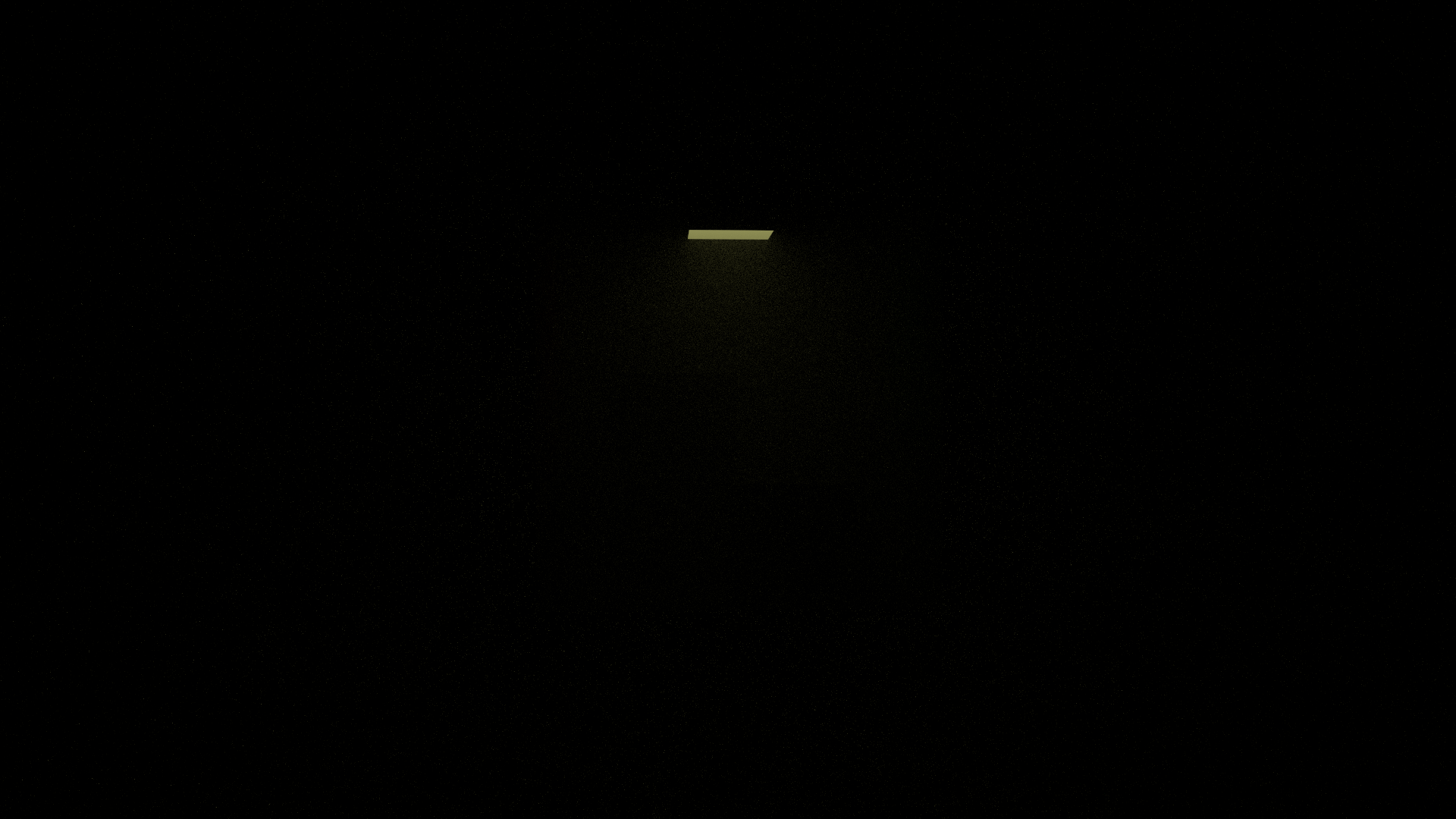
25 Despite us wanting to emulate foggy, it’s not like a hazy day or a foggy day where there’s a sun behind a thick layer of scattering, but think of it as foggy in the nighttime without moonlight or stars (i.e., it’s just goign to be pitch black).
24 The sensor importance that corresponds to the physical process of vignetting. There’s an additional factor of \(\frac{1}{z^2}\) where \(z\) is the normal distance between the pinhole aperature and the sensor surface/window (i.e., depth). Since majority of the cases \(z=1\), we can ignore it and leave just the \(\cos\) term.
I think I know how to live in harmony with AI coding tools now. Writing the algorithm to actually learn what you are doing without the slowdown of fixing errors, bugs, and dealing with syntax. Now, I can finally play around the coefficients in peace and have fun. (There’s not much to play around with this basic model.) As you play around more, you would realize the the “god” rays are very noise (i.e., high variance). There must be a better way and I hope I can improve it later down the line. For now, there’s other aspect of volumetric rendering I want to explore (i.e., inhomogenous medium and fluid simulation).
Visual Results!
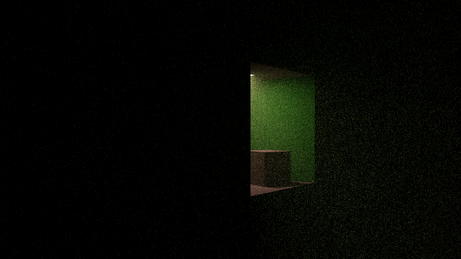
Note: When I originally render the medium, it was pitch black. Due to how everything is “far apart” in my scene (i.e., on a order of 100s), the range of coefficients is much different. In fact, it has to be on a level of thousandths or ten-thousandths, and somewhat sensitive to changes in the coefficient. Just something to be aware.
Source code: https://github.com/andrew-shc/vpt.